Using The Panel Study Of Income Dynamics
What is the PSID?
The Panel Study of Income Dynamics (PSID) is a longitudinal public dataset which has been following a collection of families and their descendants since 1968. It provides a breadth of information about labor supply, family structure, health, and life-cycle dynamics. More information is available at https://psidonline.isr.umich.edu/.
Structure of the PSID data
The PSID consists mainly of two sets of data: the individuals file and the family files. Each row of the individual file describes an individual who appears at some point in the PSID data. The values list each year this person is available, and the code of the family they appear in that year.
The main data comes from the family files, one for each year. Within a file, each row is a family. For single families, the main adult is considered the household head, and variables like “head income” refer to this person. For married families, there is a household head and a household spouse. Usually there are variables for each of them, like “head income” and “spouse income”.
The PSID data center is the source of the data. However, it isn’t easy to produce a panel dataset using the data center. The dataset it produces leaves variables with names like ER13004, leaving you to rename the variables manually. My package PSID.jl automates this process. It also produces consistent category labels across all years, codes missing values, and assigns data from the family files to the correct individual.
All individuals appear in the data produced by PSID.jl on their own row. For example, if Alice and Bob are married, there will be two rows for their family per year. Suppose Bob is the household head. For his row, “income_ind” refers to him, and “income_spouse” refers to Alice. This data would come from the variables for “head income” and “spouse income” in the family file. For Alice’s row, this is reversed. “income_ind” refers to her, and “income_spouse” refers to Bob.
Using PSID.jl
To use PSID.jl, you will first need to construct a JSON file listing the variables in the family files that you want. An example is shown below.
[
  {
    "name_user": "id",
    "varID": "V3",
    "unit": "family"
  },
  {
    "name_user": "hours",
    "varID": "V465",
    "unit": "head"
  },
  {
    "name_user": "hours",
    "varID": "V53",
    "unit": "spouse"
  },
  {
    "name_user": "state",
    "varID": "ER13004",
    "unit": "family"
  },
  {
    "name_user": "age",
    "varID": "ER60017",
    "unit": "head"
  },
  {
    "name_user": "age",
    "varID": "ER60019",
    "unit": "spouse"
  },
  {
    "name_user": "sex",
    "varID": "ER60018",
    "unit": "head"
  },
  {
    "name_user": "sex",
    "varID": "ER60020",
    "unit": "spouse"
  },
  {
    "name_user": "labor_inc",
    "varID": "ER65216",
    "unit": "head"
  },
  {
    "name_user": "labor_inc",
    "varID": "ER65244",
    "unit": "spouse"
  },
  {
    "name_user": "labor_inc_pre",
    "varID": "V75",
    "unit": "spouse"
  },
  {
    "name_user": "num_kids",
    "varID": "V398",
    "unit": "family"
  }
]
There are three fields, name_user, varID, and unit. name_user is a name chosen by you. varID is one of the codes assigned by the PSID to this variable. These can be looked up in the PSID cross-year index. For example, hours above can be found in the crosswalk at Family Public Data Index 01>WORK 02>Hours and Weeks 03>annual in prior year 04>head 05>total:. Clicking on the variable info will show the the list of years and associated IDs when that variable is available. Choose any of the IDs for varID, it does not matter. PSID.jl will look up all available years for that variable in the crosswalk. You must also indicate the unit, which can be head, spouse, or family. This makes sure the variable is assigned to the correct individual.
Next, you will need to download the data files manually. This requires creating a free PSID account, so I can’t distribute them automatically. It should only take you 5 minutes to download the files. See my instructions for how to do this.
Finally, make sure the user_input.json and the data files are in the same directory. Launch
Julia in that directory, and execute these commands.
using PSID
makePSID("user_input.json")
After a few minutes, you’ll see a message Finished constructing individual data, saved to output/allinds.csv.
Using the PSID
You can use the allinds.csv you just generated in whatever statistical software you want. I will
analyze the PSID data using Julia and the DataFrames and StatsPlots packages.
First, let’s activate our project and read our data.
using InstantiateFromURL
github_project("aaowens/aaowens.github.io", path = "_misc/PSID", force = true)
Info Local TOML exists; removing now.
Activating environment at `~/Documents/data/myblog/aaowens.github.io/_posts
_content/Project.toml`
Precompiling project...
Info Project name is NA, version is NA
using DataFrames, CSV, DataFramesMeta, StatsPlots, Missings
alldata = CSV.read("output/allinds.csv", copycols = true);
Next, we can look at a few columns.
head(alldata[:, 1:4])
6×4 DataFrames.DataFrame
│ Row │ id_ind │ famid_1968 │ year  │ id_family │
│     │ Int64  │ Int64      │ Int64 │ Float64   │
├─────┼────────┼────────────┼───────┼───────────┤
│ 1   │ 1001   │ 1          │ 1968  │ 1.0       │
│ 2   │ 2001   │ 2          │ 1968  │ 2.0       │
│ 3   │ 3001   │ 3          │ 1968  │ 3.0       │
│ 4   │ 4001   │ 4          │ 1968  │ 4.0       │
│ 5   │ 5001   │ 5          │ 1968  │ 5.0       │
│ 6   │ 6001   │ 6          │ 1968  │ 6.0       │
head(alldata[:, 9:10])
6×2 DataFrames.DataFrame
│ Row │ educ_ind │ educ_ind_code_ind │
│     │ Float64⍰ │ String⍰           │
├─────┼──────────┼───────────────────┤
│ 1   │ 8.0      │ ER30010           │
│ 2   │ 3.0      │ ER30010           │
│ 3   │ 0.0      │ ER30010           │
│ 4   │ 8.0      │ ER30010           │
│ 5   │ 10.0     │ ER30010           │
│ 6   │ 8.0      │ ER30010           │
In the above example, id_ind is ID of this individual. id_ind and year uniquely
identify the rows, forming the panel structure. educ_ind is the years of education for this individual, while
educ_ind_code_fam is the code of this variable in the family file. This code changes
every year. You can search for this code in the PSID data center to obtain the exact
description of this variable.
Next, we check the number of observations, which is the number of (individual, year) pairs in the data. We also describe the dataset.
println("$(nrow(alldata)) rows")
458192 rows
describe(alldata, :nmissing)
41×2 DataFrames.DataFrame
│ Row │ variable                   │ nmissing │
│     │ Symbol                     │ Union…   │
├─────┼────────────────────────────┼──────────┤
│ 1   │ id_ind                     │          │
│ 2   │ famid_1968                 │          │
│ 3   │ year                       │          │
│ 4   │ id_family                  │          │
│ 5   │ id_family_code_ind         │          │
│ 6   │ rel_head_ind_label         │          │
│ 7   │ rel_head_ind               │          │
⋮
│ 34  │ sex_spouse                 │ 283052   │
│ 35  │ sex_spouse_code_fam        │ 273873   │
│ 36  │ labor_inc_spouse           │ 241688   │
│ 37  │ labor_inc_spouse_code_fam  │ 162297   │
│ 38  │ labor_inc_pre_ind          │ 392963   │
│ 39  │ labor_inc_pre_ind_code_fam │ 357439   │
│ 40  │ seq_num_ind                │ 7878     │
│ 41  │ seq_num_ind_code_ind       │ 7878     │
Sample selection
We need to do a small amount of data cleaning. The PSID slightly changed
the definition of labor income for spouses in 1993, so I had to pull two variables
in the JSON file above, labor_inc and labor_inc_pre. I combine these below.
I also keep only the main, representative PSID sample, dropping the SEO oversample
of low-income households. Finally, I assume labor income is 0 if it’s missing.
inds = (alldata.year .<= 1993) .& (alldata.ishead .== true)
alldata.labor_inc_spouse[inds] .= alldata.labor_inc_pre_spouse[inds]
inds = (alldata.year .<= 1993) .& (alldata.ishead .== false)
alldata.labor_inc_ind[inds] .= alldata.labor_inc_pre_ind[inds]
re(x, val) = Missings.replace(x, val) |> collect # Replace missing with value
alldata = @where(alldata, :famid_1968 .< 3000) # Keep only SRC sample
alldata.labor_inc_ind = re(alldata.labor_inc_ind, 0.)
alldata.hours_ind = re(alldata.hours_ind, 0.)
## The PSID didn't start asking the sex of the spouse until 2015 (It was assumed female)
alldata.sex_ind = re(alldata.sex_ind, 2); # Female if missing
Analyzing the data: Age profile of income
Let’s look at people’s income. This is the Panel Study of Income Dynamics after all. We want to look at the age profile of income. Since we are comparing people at very different time periods, we need to use real (inflation adjusted) income. I pull the PCE price index from FRED using FredData. I also pull per-capita aggregate income for comparison purposes.
using FredData, Dates
using StatsBase
f = Fred(FREDKEY)
a = get_data(f, "PCEPILFE", frequency = "a", units = "lin")
inflation = a.data[:, [:date, :value]]
inflation.date = inflation.date .|> Dates.year
rename!(inflation, [:value => :PCE, :date => :year])
inflation.PCE = inflation.PCE ./ 100
a = get_data(f, "A792RC0Q052SBEA", frequency = "a", units = "lin")
inc_capita = a.data[:, [:date, :value]]
inc_capita.date = inc_capita.date .|> Dates.year
rename!(inc_capita, [:value => :inc_capita, :date => :year])
alldata = join(alldata, inflation, on = :year)
alldata = join(alldata, inc_capita, on = :year)

d = alldata[:, [:id_ind, :year, :ishead, :labor_inc_ind, :hours_ind, :age_ind,
:sex_ind, :PCE, :inc_capita, :num_kids_family]]
dropmissing!(d)
d = filter(r -> r.labor_inc_ind < 2e6, d) # Drop outlier income
d = @transform(d, labor_inc_ind_real = :labor_inc_ind ./ :PCE)
d = @transform(d, inc_capita_real = :inc_capita ./ :PCE);
After sample selection, we have
using Pipe
@pipe length(unique(d.id_ind)) |> println("$_ people")
gap(A) = (x = extrema(A); x[2] - x[1])
@pipe by(d, :id_ind, :year => x -> size(x, 1)).year_function |> mean |> println("On average $_ observations per person")
@pipe by(d, :id_ind, :year => x -> gap(x)).year_function |> mean |> println("First to last observation is on average $_ years");
20153 people
On average 13.014141815114375 observations per person
First to last observation is on average 16.566764253461024 years
We’re now ready to plot our data. Let’s look at average income over time, and compare it to the aggregate figures.
@df by(d, :year, :labor_inc_ind_real => mean) plot(:year, :labor_inc_ind_real_mean, label = "PSID")
@df by(d, :year, :inc_capita_real => mean) plot!(:year, :inc_capita_real_mean,
title = "Income over time", label = "FRED", legend = :topleft)
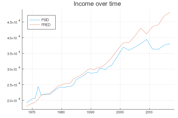
The aggregate data tracks the PSID data fairly well, which is a good sign that we haven’t made any major mistakes. I wouldn’t expect a perfect match because the PSID sample is not a simple random sample of the population, and the definitions of income are different – in the PSID I only include labor income.
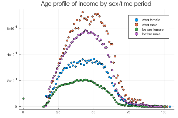
We can also look at lifecycle income. Here’s income versus age, for men and women, before and after 2000.
d.yg = ifelse.(d.year .< 2000, "before", "after")
d.sex_ind = ifelse.(d.sex_ind .== 2, "female", "male")
@df by(d, [:age_ind, :yg, :sex_ind], :labor_inc_ind_real => mean) scatter(:age_ind,
:labor_inc_ind_real_mean, group = (:yg, :sex_ind), title = "Age profile of income by sex/time period")
Lifecycle dynamics
The pictures above are interesting, but we could have produced them using cross-sectional data like the Census or CPS data. The PSID is a long panel, which means we can look at the same people when they are in their 30’s and in their 50’s. Also, because the PSID adds new individuals every year, we can see how lifecycle dynamics have changed over time, something you can’t do with cohort studies like the NLSY79. Below, I plot the joint distribution of income in 30’s versus the same individual’s income in their 50’s. I restrict the sample to men since they have higher labor-force attachment rates, especially in the earlier parts of the sample.
inrange(x, l, u) = l <= x <= u
d2 = copy(d)
# In 1997 the PSID is only collected every 2 years, not 1
# I keep only odd years over the entire sample to make sure
# the time frequency isn't influencing the results
d2 = @where(d2, isodd.(:year))
d2 = @where(d2, :sex_ind .== "male")
d2 = @where(d2, inrange.(d2.age_ind, 30, 40) .| inrange.(d2.age_ind, 50, 60))
d2.agegroup = ifelse.(d2.age_ind .<= 40, "Young", "Not_young" )
gd2 = by(d2, [:id_ind, :agegroup], :labor_inc_ind_real => mean)
wide = unstack(gd2, :id_ind, :agegroup, :labor_inc_ind_real_mean) |> dropmissing
@df wide histogram2d(:Young, :Not_young, xlabel = "Young", ylabel = "Middle",
xlims = (0, 300_000), ylims = (0, 300_000))
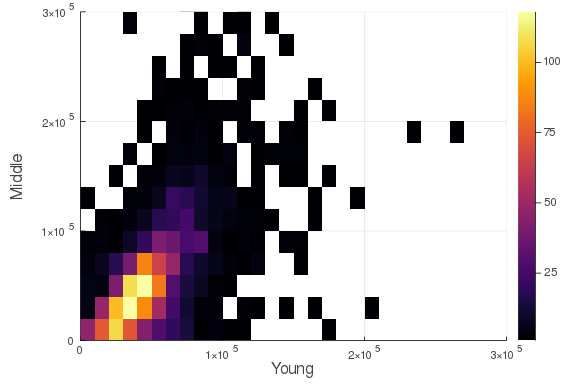
This is interesting. Unsurprisingly, income when young is positively correlated with income when middle-aged, but there is plenty of variation. Doing well in your 30’s doesn’t mean you are guaranteed to do well in your 50’s.
Lifecycle dynamics by cohort
It’s clear that income in your 50’s is correlated with income in your 30’s, but has this relationship changed over time? This question has important implications for equality of opportunity. If the correlation is very high, a rich young person knows their income is likely safe for life, but a poor young person would have little hope for advancement.
Below, I compute the correlation between 30’s income and 50’s income over time. We have to stop in 2001 because cohorts after that are too young to have data from their 50’s.
using Statistics
joinby(df, on, f...) = join(df, by(df, on, f...), on = on)
function compute_cor(window, d)
  d2 = copy(d)
  # In 1997 the PSID is only collected every 2 years, not 1
  # I keep only odd years over the entire sample to make sure
  # the time frequency isn't influencing the results
  d2 = @where(d2, isodd.(:year))
  d2 = @where(d2, :sex_ind .== "male")
  d2 = @where(d2, inrange.(d2.age_ind, 30, 40) .| inrange.(d2.age_ind, 50, 60))
  d2.agegroup = ifelse.(d2.age_ind .<= 40, "Young", "Not_young" )
  gd1 = joinby(d2, :id_ind, :year => minimum)
  gd1 = @where(gd1, :year_minimum .∈ Ref(window))
  gd2 = by(gd1, [:id_ind, :agegroup], :labor_inc_ind_real => mean)
  wide = unstack(gd2, :id_ind, :agegroup, :labor_inc_ind_real_mean) |> dropmissing
  c = corspearman(wide.Young, wide.Not_young)
  return (corr = c,)
end

yearrange = 1968:1999
c = [compute_cor(i:(i+4), d).corr for i in yearrange]
plot(yearrange, c, title = "Income correlation over time", label = "Spearman's rho",
legend = :topleft)
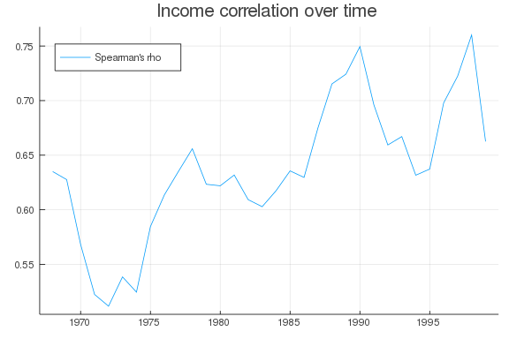
It looks like the correlation has been rising over time, so there is less opportunity for a young person to change their fortunes later in life.