Demonstrating Monte Carlo With The 538 Model
Forecasting the Democratic primary
This post is inspired by the new FiveThirtyEight primary forecast. It might be tempting to forecast the likely outcome of the primary by looking at the current polls, where they ask people who they would vote for today. As Nate Silver describes in the description of their forecast, this approach ignores a lot of complicated nonlinear dynamics. Reality has path dependence: candidates may drop out, there are discrete thresholds like requiring at least 15% of the vote in a caucus, and a candidate’s “momentum” influences their future success.
One of the more insightful comments in Silver’s post is that their forecast gives Joe Biden only a 60% chance of winning Delaware, his home state where he is very popular. In fact, were the election held today he would have an almost 100% chance of winning Delaware. The problem is that Delaware votes relatively late, and it’s possible Biden will have dropped out of the race by that point. This is nonlinear path dependence in action. In a scenario where he’s still in the race, he gets most of the vote, but he gets no votes if he’s dropped out.
Our goal in a forecast is to describe not just the most likely outcome, but quantify our uncertainty with a probability distribution. It would be very hard to capture these dynamics with a model that could be solved analytically. This is why the FiveThirtyEight forecast uses Monte Carlo simulation with a realistic model. As described in the post, they carefully model the reality of how the voting process actually works, along with a lot of assumptions about people’s voting behavior. They then run thousands of simulations with the model. Each simulation is a hypothetical reality. If we plotted a thousand paths of Joe Biden’s vote share, we’d see he usually does well once Delaware is reached, but on a few hundred paths something happened early on and he dropped out.
Monte Carlo simulations allow us to generate probability distributions of highly complex situations without that much effort. In this post, I create a model of the Democratic primary which is much simpler than the FiveThirtyEight model, but still incorporates the features I talked about. The voting mechanics in the model works as follows:
- Candidates need 50% of the total vote share to win the election.
- States vote sequentially.
- All states are caucus states, so any candidate with <15% of the vote has their vote distributed to other candidates. In reality this truncation occurs at the precinct level, but this is a simplification.
I also need to model voting behavior:
- Candidates have some base level of support
- At each election, there are IID random shocks
- Candidates have “momentum”, which I model as a random walk.
- If a candidate drops out or doesn’t meet the threshold, their votes are evenly distributed amongst the other candidates.
- Candidates drop out after the race looks hopeless. I define this as them having less than 15% of the current vote share, checking only after the first 20 states have voted.
Coding the model
Even though the resulting dynamics will be complicated, coding the model is pretty simple. Here I specify the model primitives. The base support is also a model primitive, and will be fixed in each simulation. Understanding what’s random and what’s not is important. We’re running thousands of simulations of this primary, not simulations of thousands of unrelated primaries.
These parameters I chose are pretty arbitrary. The FiveThirtyEight model, in addition to being much more realistic, calibrates their parameters based on current polling data and the results of historical primaries. They also update the forecast in real-time as new data arrives. It’s an impressive undertaking.
const N_cand = 6 # 6 candidates
const N_state = 50 # 50 states
const N_dropout = 20 # Drop out after 20 states
const cutoff = 0.15 # Caucus cutoff, truncate vote to 0
const α_momentum = 0.5 # Importance of random walk component
const α_eps = 0.3 # Importance of random shocks
using Random
Random.seed!(2)
const base = [1.2, 0.8, 0.4, -0.2, -0.5, -1];
We need to implement the vote distribution behavior. This is a little more complicated than it seems. The order in which the candidates are eliminated matters. If candidate 1 and candidate 2 both have < 10% support, eliminating candidate 1 may save candidate 2.
function distribute_vote(shares)
    newshares = copy(shares)
    for i in 1:N_cand
        if newshares[i] < cutoff # Need to distribute this person's vote
            votetotal = newshares[i]
            newshares[i] = 0
            num_takers = count(x -> x > 0, newshares) # How many people should receive vote
            for j in 1:N_cand
                if newshares[j] != 0
                    newshares[j] += votetotal / num_takers
                end
            end
        end
    end
    newshares
end;
Now we’re ready to implement our simulation
function simulate()
    votes = zeros(N_cand, N_state)
    dropped_out = zeros(Bool, N_cand)
    momentum = zeros(N_cand)
    # The simulation
    for t in 1:N_state # For each state
        eps = α_eps * randn(N_cand) # Draw shocks
        momentum .+= α_momentum .* randn(N_cand)
        vote = exp.(base .+ eps .+ momentum) # Votes must be positive, so use exp
        for i in 1:N_cand
            if dropped_out[i] # If they dropped out, take away their votes
                vote[i] = 0
            end
        end
        shares = vote ./ sum(vote) # Vote shares sum to 1
        shares = distribute_vote(shares) # Apply the caucus rules
        votes[:, t] = shares
        cvotes = cumsum(votes, dims = 2)
        # Check if anyone should drop out
        if t > N_dropout # Need at least N_dropout of history to check this
            for i in 1:N_cand
                # We divide by t here to convert from total votes to the vote share
                cvotes[i, t] / t <= (cutoff) && (dropped_out[i] = true) # Race is hopeless
            end
        end
    end
    return votes
end;
To check how our simulation works, let’s plot a sample primary with a 50% goalpost marker.
using Plots
using Random
Random.seed!(1)
votes = simulate()
cvotes = cumsum(votes, dims = 2) / sum(votes)
plot(cvotes')
plot!(1:50, 0.5*ones(50), legend = false)
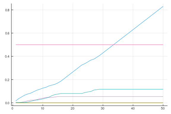
In this sample, the blue candidate won easily. Everyone else drops out fairly early.
Now we are ready to do Monte Carlo. I simulate 100 primaries and plot candidate 1’s total votes for each one.
votesim = [simulate() for i = 1:100]
paths = [cumsum(votes, dims = 2) for votes in votesim]
pathA = reduce(hcat, [path[1, :] for path in paths])
plot(pathA / N_state)
plot!(1:N_state, (0.5)*ones(N_state), legend = false)
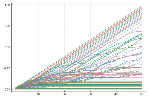
The dynamics I discussed above are reflected here. In many cases, this candidate simply has a poor start and drops out early. The simulated data tells us the entire (approximate) distribution of outcomes. We can use it to compute any statistic we want. The most obvious question is, who will win the primary? We compute that by counting the number of times each candidate wins.
using StatsBase
function winner(path)
    x = findfirst(x -> x > 0.5 * N_state, path[:, N_state]) # Index of the winner, if any
    out = x === nothing ? 0 : x # Julia outputs nothing if there was no match
end
StatsBase.proportionmap(winner.(paths))
Dict{Int64,Float64} with 7 entries:
  0 => 0.17
  4 => 0.07
  2 => 0.17
  3 => 0.16
  5 => 0.09
  6 => 0.03
  1 => 0.31
This tells us that candidate 1 has a 31% chance of winning the primary. Still, even the weakest candidate wins 3% of the time. The number 0 represents that no candidate won a majority.
Conditioning
Coming back to the example where Joe Biden may lose Delaware, we can condition our simulation on some event. It’s easy to condition when doing Monte Carlo. Simply exclude all paths where that event didn’t happen, and do your analysis as if that were the universe of possible paths. Let’s condition on the event that candidate 1 has less than 30% of the current vote share after the 10th state.
votesim = [simulate() for i = 1:100]
votesim_cond = filter(votesim) do votes
    path = cumsum(votes, dims = 2)
    path[1, 10] / 10 <= 0.3
end
paths = [cumsum(votes, dims = 2) for votes in votesim_cond]
pathA = reduce(hcat, [path[1, :] for path in paths])
plot(pathA / N_state)
plot!(1:N_state, (0.5)*ones(N_state), legend = false)
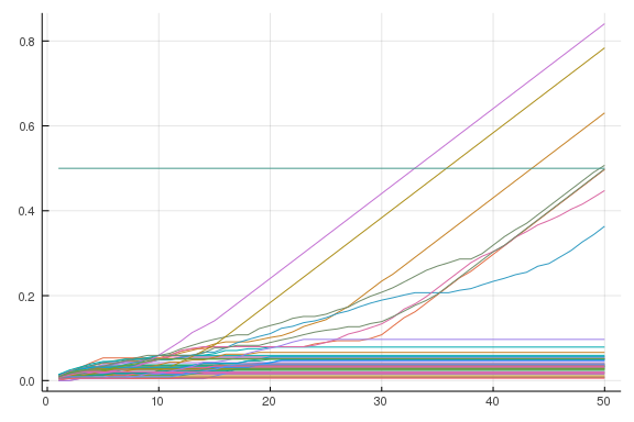
We see that if candidate 1 has a poor start, he likely drops out. However, it is not entirely hopeless. In a few of the paths he bounces back.
Who would benefit from candidate 1’s misfortune?
StatsBase.proportionmap(winner.(paths))
Dict{Int64,Float64} with 7 entries:
  0 => 0.191489
  4 => 0.0425532
  2 => 0.297872
  3 => 0.212766
  5 => 0.148936
  6 => 0.0212766
  1 => 0.0851064
Candidate 2 goes from a 17% chance to a 30% chance of winning in this situation.