Parallel Value Function Iteration In Julia
Serial
Here we perform a serial (single-core) value function iteration to solve a simple savings problem with idiosyncratic income shocks. To solve the Bellman equation at each point in the state space, we use numerical optimization (Brent’s method) and monotonic cubic spline interpolation over the expected value function. For simplicity we iterate a fixed 100 times.
using InstantiateFromURL
github_project("aaowens/aaowens.github.io", path = "_misc/ParallelVFI", force = true)
Info Local TOML exists; removing now.
Activating environment at `~/Documents/data/myblog/aaowens.github.io/_posts
_content/Project.toml`
Precompiling project...
Info Project name is NA, version is NA
using Interpolations, Optim, BenchmarkTools, QuantEcon
const agrid = exp.(range(log(1), stop = log(200), length = 100 )) .- 1
uc(c) = c > 0 ? c^(-2.5)/-2.5 : -Inf
u(a, ap, x) =  uc(a - ap + x)
maxap(a, x) = a + x
const beta = 0.96
using Random
Random.seed!(2)
mc = QuantEcon.tauchen(20, .8, .5)
const P = mc.p
const xgrid = exp.(mc.state_values) .+ 0.1
20-element Array{Float64,1}:
  0.18208499862389876
  0.20679522050714869
  0.23894401308852461
  0.2807706251409615
  0.3351883912625588
  0.40598765336756437
  0.4980997680657806
  0.6179405887454282
  0.77385734679864
  0.9767100584536119
  1.240627953743172
  1.583993614896087
  2.030723372003401
  2.61193313891799
  3.3681057192812967
  4.351910541297183
  5.631872223267574
  7.297143495221169
  9.463714923300914
 12.282493960703478
# Bellman step given evf and x
function bellman(evf, x)
    vf, pol = similar(evf), similar(evf)
    for i in eachindex(vf)
        a = agrid[i]
        obj = ap -> -(u(a, ap, x) + beta * evf(ap))
        upper = min(maxap(a, x), agrid[end])
        sol = optimize(obj, agrid[1], .99*upper)
        vf[i], pol[i] = -sol.minimum, sol.minimizer
    end
    return vf, pol
end

function expectation(bigvf, P)
   evf = similar(bigvf)
    for a_nx in 1:size(bigvf, 1)
        for x_nx in 1:size(P, 1)
        ev = 0.
            for xp_nx in 1:size(P, 2)
                ev += bigvf[a_nx, xp_nx] * P[x_nx, xp_nx]
            end
            evf[a_nx, x_nx] = ev
        end
    end
    return evf
end
expectation (generic function with 1 method)
vfall = zeros(length(agrid), length(xgrid))
polall = zeros(length(agrid), length(xgrid))
function test_serial(vfall, polall)
   fill!(vfall, 0) # reset the value function each time we benchmark
   fill!(polall, 0)
   for i in 1:100
      vfe = expectation(vfall, P)
      for x_nx in eachindex(xgrid)
         vfold = interpolate(agrid, vfe[:, x_nx], SteffenMonotonicInterpolation())
         vf, pol = bellman(vfold, xgrid[x_nx])
         vfall[:, x_nx] = vf; polall[:, x_nx] = pol
      end
   end
   return vfall, polall
end
vfall, polall = test_serial(vfall, polall)
@time vfall, polall = test_serial(vfall, polall);
0.419485 seconds (618.11 k allocations: 53.327 MiB, 3.48% gc time)
Threads
Here we use multithreading. See https://docs.julialang.org/en/v1/manual/parallel-computing/#Setup-1 for how to enable this. There is no interaction between loop iterations, so this is thread-safe. We check the output at the end.
vfall2 = zeros(length(agrid), length(xgrid))
polall = zeros(length(agrid), length(xgrid))
function test_threads(vfall, polall)
    fill!(vfall, 0) # reset the value function each time we benchmark
    fill!(polall, 0)
    for i in 1:100
        vfe = expectation(vfall, P)
        Threads.@threads for x_nx in eachindex(xgrid)
            vfold = interpolate(agrid, vfe[:, x_nx], SteffenMonotonicInterpolation())
            vf, pol = bellman(vfold, xgrid[x_nx])
            vfall[:, x_nx] = vf; polall[:, x_nx] = pol
        end
    end
    return vfall, polall
end
vfall, polall = test_threads(vfall2, polall)
@time vfall, polall = test_threads(vfall2, polall);
0.433563 seconds (619.01 k allocations: 53.406 MiB, 3.02% gc time)
all(vfall .== vfall2) #did multithreading give the same result as serial?
true
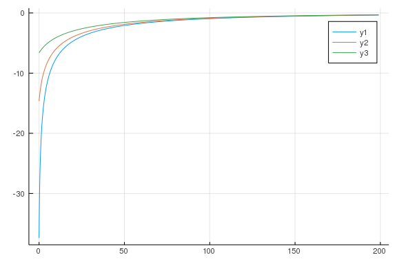
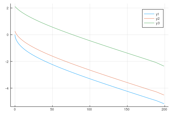
Threads is about 4x faster than serial with 4 threads. To check that we solved the model correctly, let’s plot the output.
using Plots
# net savings
p1 = plot(agrid, polall[:, 1] .- agrid)
plot!(agrid, polall[:, 10] .- agrid)
plot!(agrid, polall[:, 15] .- agrid)
# value
plot(agrid, vfall[:, 5])
plot!(agrid, vfall[:, 10])
plot!(agrid, vfall[:, 15])